class: center, middle, inverse, title-slide # ASP 460 2.0 Data Visualization ### Dr Thiyanga Talagala ### Principal Component Analysis --- # PCA - Finding low-dimensional combinations (or projections) of high dimensional data that capture most of the variability in the original data. - Objective: Take `\(P\)` variables `\(X_1, X_2, X_3,...X_p\)` and find combinations of these to produce variables (components) `\(Z_1, Z_2...Z_p\)` that are uncorrelated. > Number of PCs = Number of variables in the original data. - The components are ordered so that `\(Z_1\)` captures the largest proportion of the data, `\(Z_2\)` captures the next largest proportion of the variability > `\(Var(Z_1) \geq Var(Z_2)...\geq Var(Z_p)\)` --- # PCA (cont.) - If original variables are uncorrelated then PCA does nothing at all. The PCs are the same as the original data. - PCs are formed by calculating the eigen vectors and eigen values of the data covariance matrix. --- # Data ``` Rows: 344 Columns: 8 $ species <fct> Adelie, Adelie, Adelie, Adelie, Adelie, Adelie, Adel… $ island <fct> Torgersen, Torgersen, Torgersen, Torgersen, Torgerse… $ bill_length_mm <dbl> 39.1, 39.5, 40.3, NA, 36.7, 39.3, 38.9, 39.2, 34.1, … $ bill_depth_mm <dbl> 18.7, 17.4, 18.0, NA, 19.3, 20.6, 17.8, 19.6, 18.1, … $ flipper_length_mm <int> 181, 186, 195, NA, 193, 190, 181, 195, 193, 190, 186… $ body_mass_g <int> 3750, 3800, 3250, NA, 3450, 3650, 3625, 4675, 3475, … $ sex <fct> male, female, female, NA, female, male, female, male… $ year <int> 2007, 2007, 2007, 2007, 2007, 2007, 2007, 2007, 2007… ``` ``` species island bill_length_mm bill_depth_mm Adelie :152 Biscoe :168 Min. :32.10 Min. :13.10 Chinstrap: 68 Dream :124 1st Qu.:39.23 1st Qu.:15.60 Gentoo :124 Torgersen: 52 Median :44.45 Median :17.30 Mean :43.92 Mean :17.15 3rd Qu.:48.50 3rd Qu.:18.70 Max. :59.60 Max. :21.50 NA's :2 NA's :2 flipper_length_mm body_mass_g sex year Min. :172.0 Min. :2700 female:165 Min. :2007 1st Qu.:190.0 1st Qu.:3550 male :168 1st Qu.:2007 Median :197.0 Median :4050 NA's : 11 Median :2008 Mean :200.9 Mean :4202 Mean :2008 3rd Qu.:213.0 3rd Qu.:4750 3rd Qu.:2009 Max. :231.0 Max. :6300 Max. :2009 NA's :2 NA's :2 ``` --- # Data Cleaning ``` # A tibble: 6 × 8 species island culmen_length culmen_depth flipper_length body_mass sex year <fct> <fct> <dbl> <dbl> <int> <int> <fct> <int> 1 Adelie Torge… 39.1 18.7 181 3750 male 2007 2 Adelie Torge… 39.5 17.4 186 3800 fema… 2007 3 Adelie Torge… 40.3 18 195 3250 fema… 2007 4 Adelie Torge… 36.7 19.3 193 3450 fema… 2007 5 Adelie Torge… 39.3 20.6 190 3650 male 2007 6 Adelie Torge… 38.9 17.8 181 3625 fema… 2007 ``` ``` species island culmen_length culmen_depth flipper_length Adelie :146 Biscoe :163 Min. :32.10 Min. :13.10 Min. :172 Chinstrap: 68 Dream :123 1st Qu.:39.50 1st Qu.:15.60 1st Qu.:190 Gentoo :119 Torgersen: 47 Median :44.50 Median :17.30 Median :197 Mean :43.99 Mean :17.16 Mean :201 3rd Qu.:48.60 3rd Qu.:18.70 3rd Qu.:213 Max. :59.60 Max. :21.50 Max. :231 body_mass sex year Min. :2700 female:165 Min. :2007 1st Qu.:3550 male :168 1st Qu.:2007 Median :4050 Median :2008 Mean :4207 Mean :2008 3rd Qu.:4775 3rd Qu.:2009 Max. :6300 Max. :2009 ``` --- <!-- --> --- background-image: url('lter_penguins.png') background-size: contain .footer-note[.tiny[.green[Artwork by @allison_horst]]] --- background-image: url('culmen_depth.png') background-size: contain .footer-note[.tiny[.green[Artwork by @allison_horst]]] --- # PCA 1. Select numerical variables 2. scale the data to 0 mean and unit variance. 3. Perform PCA. --- # PCA ``` Standard deviations (1, .., p=4): [1] 1.6569115 0.8821095 0.6071594 0.3284579 Rotation (n x k) = (4 x 4): PC1 PC2 PC3 PC4 culmen_length 0.4537532 -0.60019490 -0.6424951 0.1451695 culmen_depth -0.3990472 -0.79616951 0.4258004 -0.1599044 flipper_length 0.5768250 -0.00578817 0.2360952 -0.7819837 body_mass 0.5496747 -0.07646366 0.5917374 0.5846861 ``` <!-- --> --- # Standard deviations associated with PCs ```r summary(pca) ``` ``` Importance of components: PC1 PC2 PC3 PC4 Standard deviation 1.6569 0.8821 0.60716 0.32846 Proportion of Variance 0.6863 0.1945 0.09216 0.02697 Cumulative Proportion 0.6863 0.8809 0.97303 1.00000 ``` # PCA rotation matrix ```r pca$rotation ``` ``` PC1 PC2 PC3 PC4 culmen_length 0.4537532 -0.60019490 -0.6424951 0.1451695 culmen_depth -0.3990472 -0.79616951 0.4258004 -0.1599044 flipper_length 0.5768250 -0.00578817 0.2360952 -0.7819837 body_mass 0.5496747 -0.07646366 0.5917374 0.5846861 ``` --- # Predict PCs ```r predict(pca, newdata=tail(penguins)) ``` ``` PC1 PC2 PC3 PC4 [1,] -0.4507833 -0.06535056 -0.7461058 -0.01287014 [2,] 0.5526429 -2.34408404 -0.8679388 -0.38749681 [3,] -0.7388017 -0.24778208 -0.3155918 -0.73267497 [4,] -0.3673370 -0.98959040 -0.8866618 0.19556826 [5,] 0.4916198 -1.48261810 -0.3294640 -0.55003132 [6,] -0.2130962 -1.25965815 -0.7648157 -0.10807071 ``` ```r tail(pca$x) ``` ``` PC1 PC2 PC3 PC4 328 -0.4507833 -0.06535056 -0.7461058 -0.01287014 329 0.5526429 -2.34408404 -0.8679388 -0.38749681 330 -0.7388017 -0.24778208 -0.3155918 -0.73267497 331 -0.3673370 -0.98959040 -0.8866618 0.19556826 332 0.4916198 -1.48261810 -0.3294640 -0.55003132 333 -0.2130962 -1.25965815 -0.7648157 -0.10807071 ``` --- # PCA ``` PC1 PC2 PC3 PC4 1 -1.850808 -0.03202119 0.23454869 0.5276026 2 -1.314276 0.44286031 0.02742880 0.4011230 3 -1.374537 0.16098821 -0.18940423 -0.5278675 4 -1.882455 0.01233268 0.62792772 -0.4721826 5 -1.917096 -0.81636958 0.69999797 -0.1961213 6 -1.770356 0.36567266 -0.02841769 0.5046092 ``` # Original data ``` # A tibble: 6 × 8 species island culmen_length culmen_depth flipper_length body_mass sex year <fct> <fct> <dbl> <dbl> <int> <int> <fct> <int> 1 Adelie Torge… 39.1 18.7 181 3750 male 2007 2 Adelie Torge… 39.5 17.4 186 3800 fema… 2007 3 Adelie Torge… 40.3 18 195 3250 fema… 2007 4 Adelie Torge… 36.7 19.3 193 3450 fema… 2007 5 Adelie Torge… 39.3 20.6 190 3650 male 2007 6 Adelie Torge… 38.9 17.8 181 3625 fema… 2007 ``` --- # Combine PCA + original data ```r pcadf <- data.frame(pca$x) penguins_pca <- bind_cols(penguins, pcadf) head(penguins_pca ) ``` ``` # A tibble: 6 × 12 species island culmen_length culmen_depth flipper_length body_mass sex year <fct> <fct> <dbl> <dbl> <int> <int> <fct> <int> 1 Adelie Torge… 39.1 18.7 181 3750 male 2007 2 Adelie Torge… 39.5 17.4 186 3800 fema… 2007 3 Adelie Torge… 40.3 18 195 3250 fema… 2007 4 Adelie Torge… 36.7 19.3 193 3450 fema… 2007 5 Adelie Torge… 39.3 20.6 190 3650 male 2007 6 Adelie Torge… 38.9 17.8 181 3625 fema… 2007 # … with 4 more variables: PC1 <dbl>, PC2 <dbl>, PC3 <dbl>, PC4 <dbl> ``` --- # PC1 vs PC2 <!-- --> --- # Plotting PCA ``` Standard deviations (1, .., p=4): [1] 1.6569115 0.8821095 0.6071594 0.3284579 Rotation (n x k) = (4 x 4): PC1 PC2 PC3 PC4 culmen_length 0.4537532 -0.60019490 -0.6424951 0.1451695 culmen_depth -0.3990472 -0.79616951 0.4258004 -0.1599044 flipper_length 0.5768250 -0.00578817 0.2360952 -0.7819837 body_mass 0.5496747 -0.07646366 0.5917374 0.5846861 ``` ``` [1] 68.633893 19.452929 9.216063 2.697115 ``` <!-- --> --- ## Biplot - plot each variables coefficients inside a unit circle .pull-left[ 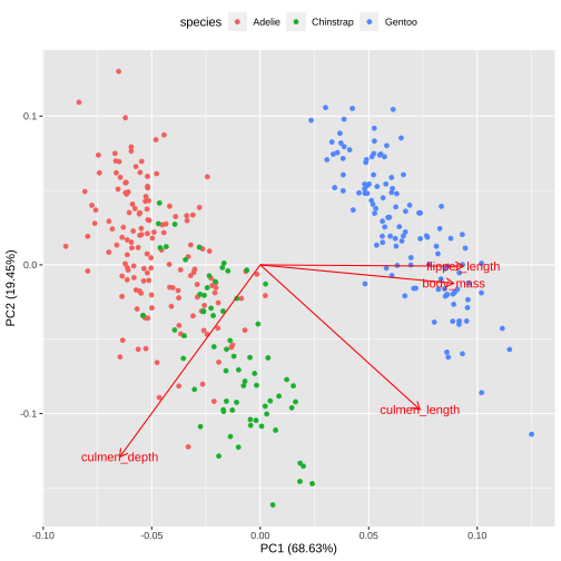<!-- --> ] .pull-right[ 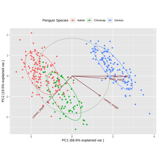<!-- --> ] PCA rotation ``` PC1 PC2 PC3 PC4 culmen_length 0.4537532 -0.60019490 -0.6424951 0.1451695 culmen_depth -0.3990472 -0.79616951 0.4258004 -0.1599044 flipper_length 0.5768250 -0.00578817 0.2360952 -0.7819837 body_mass 0.5496747 -0.07646366 0.5917374 0.5846861 ``` --- class: middle, center # Plotting PCA - PC1 --- .pull-left[ 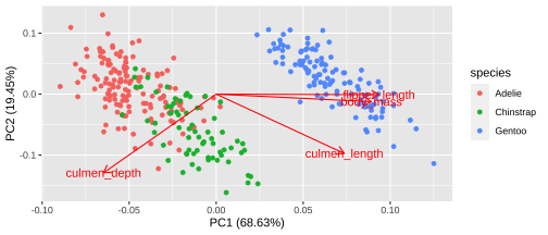<!-- -->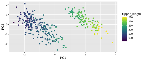<!-- --> ] .pull-right[ <!-- --> <!-- --> ] --- class: middle, center # Plotting PCA - PC1 --- .pull-left[ <!-- --><!-- --> ] .pull-right[ <!-- --> <!-- --> ] --- class: middle, center # Plotting PCA - PC2 --- .pull-left[ <!-- --><!-- --> ] .pull-right[ <!-- --> <!-- --> ] --- class: middle, center # Plotting PCA - PC2 --- .pull-left[ <!-- --><!-- --> ] .pull-right[ <!-- --> <!-- --> ] --- # Visualising instance space 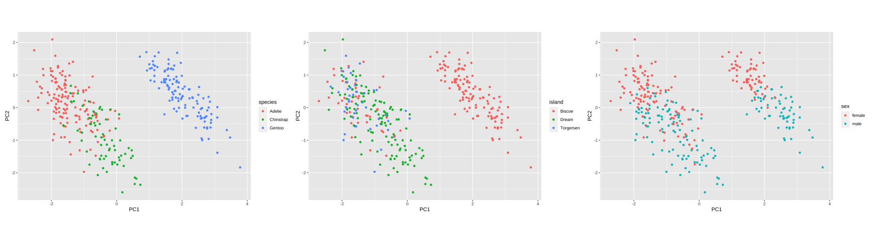<!-- -->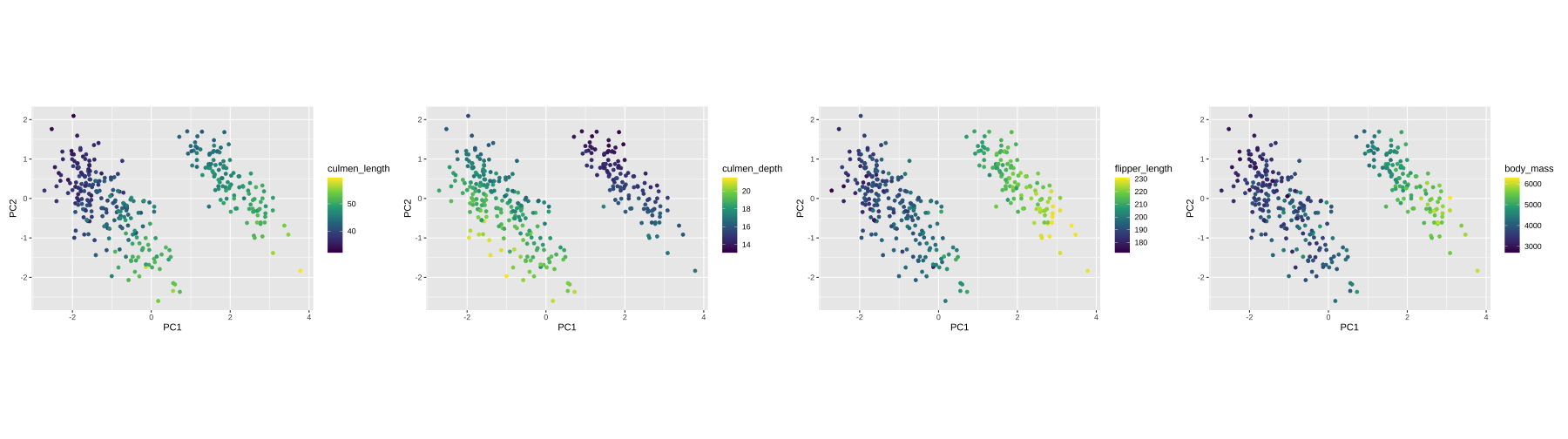<!-- -->