class: center, middle, inverse, title-slide .title[ # ASP 460 2.0 Data Visualization ] .author[ ### Dr Thiyanga Talagala ] .date[ ### Colour Scales ] --- ## Color Scales 1. Qualitative color scale 2. Sequential color scale 2. Diverging color scale --- # Qualitative color scale 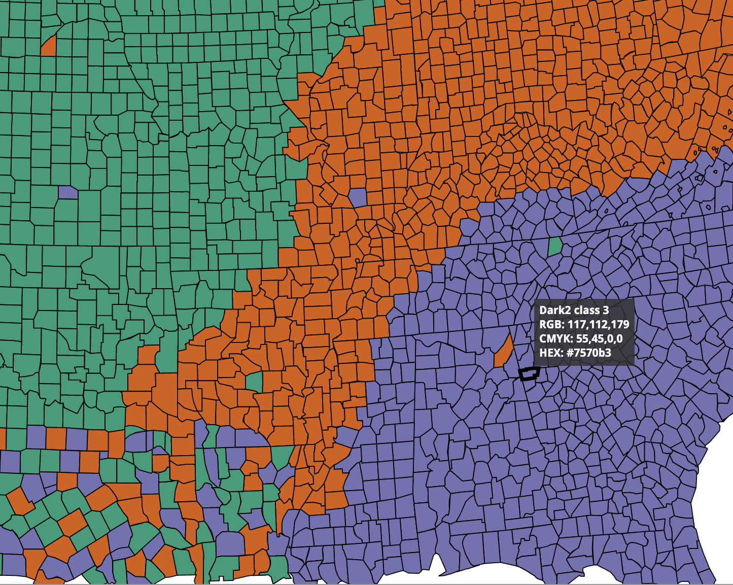 --- # Sequential color scale 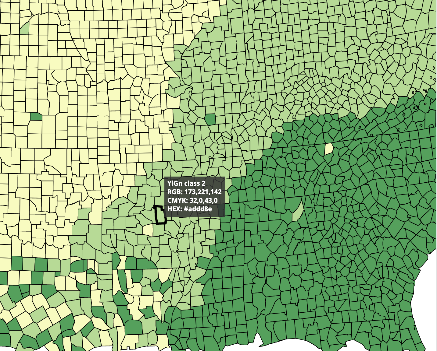 --- # Diverging color scale 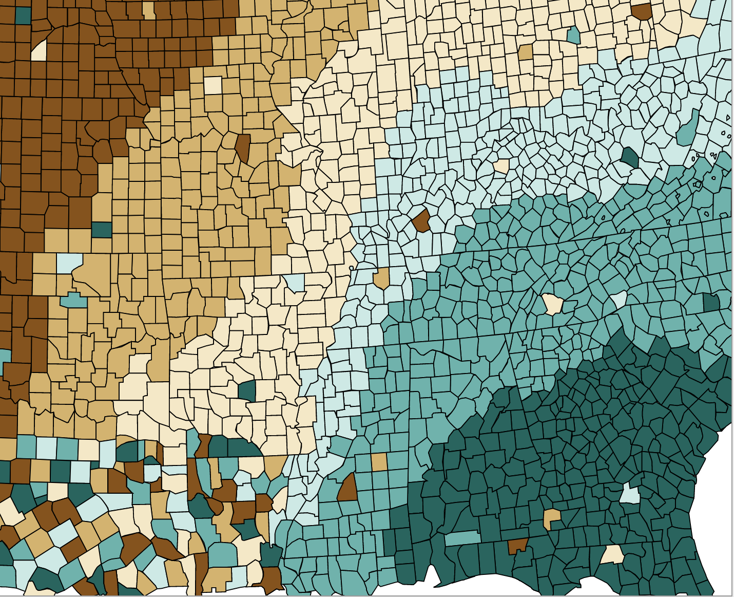 --- background-image: url(colours.png) background-size: contain --- background-image: url(tt.png) background-size: contain <!--https://www.news-medical.net/health/Classification-of-Color-Blindness-Deficiencies.aspx--> --- class: inverse, center, middle # Setting colours in ggplot --- ```r library(ggplot2) ggplot(iris, aes(x=Sepal.Length, y=Sepal.Width)) + geom_point() ``` 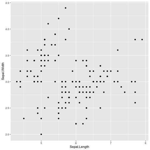<!-- --> --- ```r library(ggplot2) ggplot(iris, aes(x=Sepal.Length, y=Sepal.Width)) + geom_point(color="purple") ``` <!-- --> --- ```r library(ggplot2) ggplot(iris, aes(x=Sepal.Length, y=Sepal.Width, color=Species)) + geom_point() ``` <!-- --> --- ```r library(ggplot2) ggplot(iris, aes(x=Sepal.Length, y=Sepal.Width, color=Petal.Length < 5)) + geom_point() ``` <!-- --> --- ```r cols <- c("setosa" = "red", "versicolor" = "blue", "virginica" = "darkgreen") ggplot(iris, aes(x = Sepal.Length, y = Sepal.Width, color = Species)) + geom_point( ) + scale_colour_manual(values = cols) ``` <!-- --> --- .pull-left[ 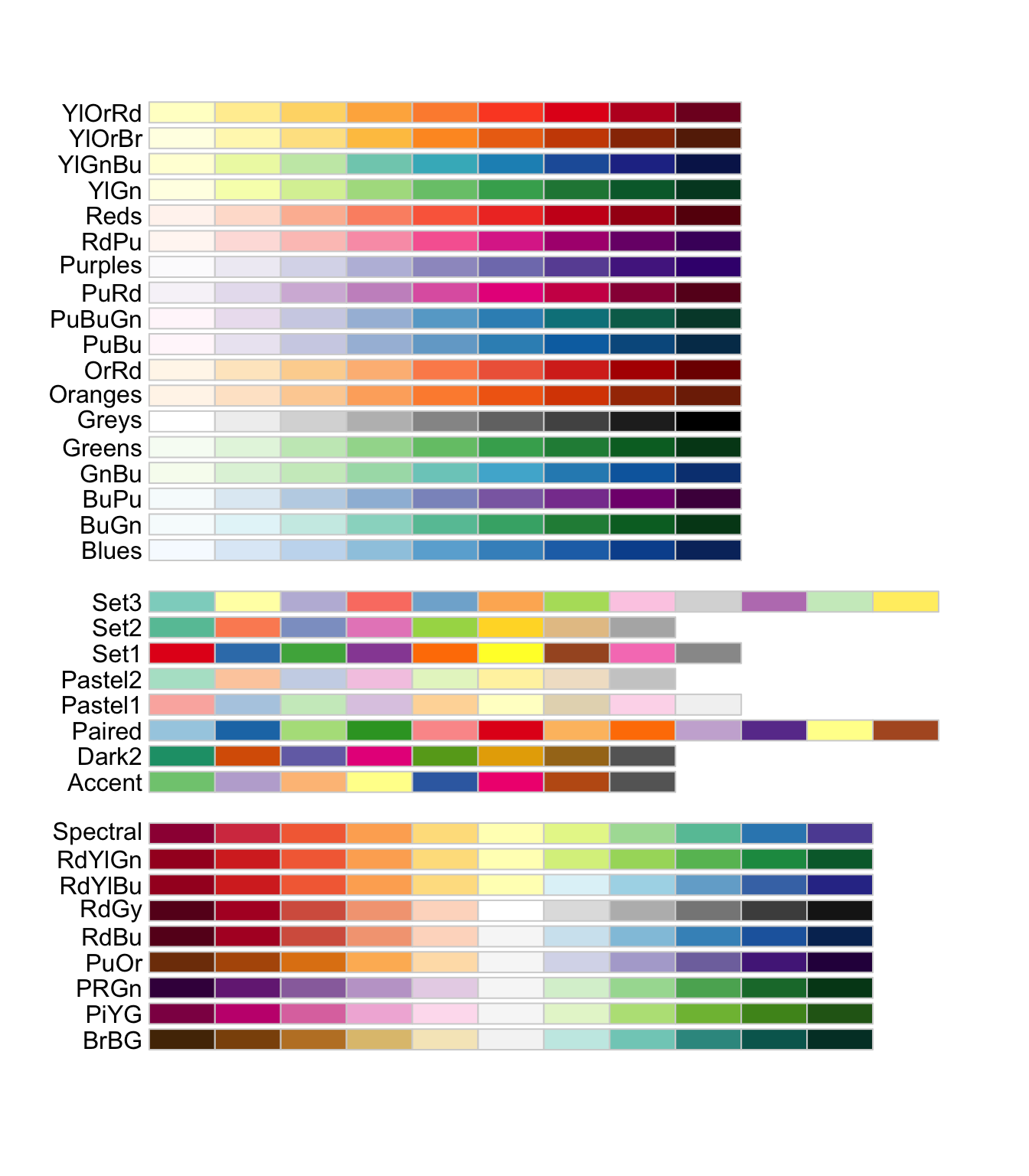 ] .pull-right[ ```r RColorBrewer::display.brewer.all() ``` - seq (sequential) - div (diverging) - qual (qualitative) ] --- ```r cols <- c("setosa" = "red", "versicolor" = "blue", "virginica" = "darkgreen") ggplot(iris, aes(x = Sepal.Length, y = Sepal.Width, color = Species)) + geom_point( ) + scale_color_brewer(type = 'qual', palette = 'Dark2') ``` <!-- --> --- background-image:url(brew.png) background-size: contain --- ```r ggplot(iris, aes(x = Sepal.Length, y = Sepal.Width, color = Species)) + geom_point( ) + scale_color_manual(values = c("#1b9e77", "#d95f02", "#7570b3")) ``` 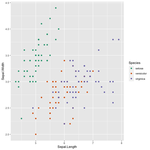<!-- --> --- # Viridis colour scales from viridisLite "The viridis scales provide colour maps that are perceptually uniform in both colour and black-and-white. They are also designed to be perceived by viewers with common forms of colour blindness. See also https://bids.github.io/colormap/." source: https://ggplot2.tidyverse.org/reference/scale_viridis.html --- ```r ggplot(iris, aes(x = Sepal.Length, y = Sepal.Width, color = Species)) + geom_point( ) + scale_colour_viridis_d() ``` 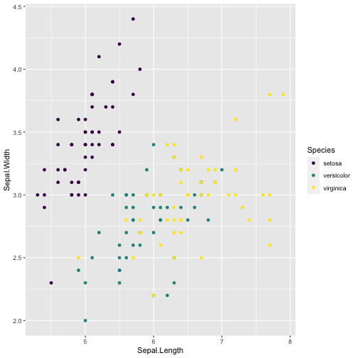<!-- --> --- ```r ggplot(iris, aes(x = Sepal.Length, y = Sepal.Width, color = Species)) + geom_point( ) + scale_colour_viridis_d(option = "plasma") ``` <!-- --> --- ```r ggplot(iris, aes(x = Sepal.Length, y = Sepal.Width, color = Species)) + geom_point( ) + scale_colour_viridis_d(option = "inferno") ``` 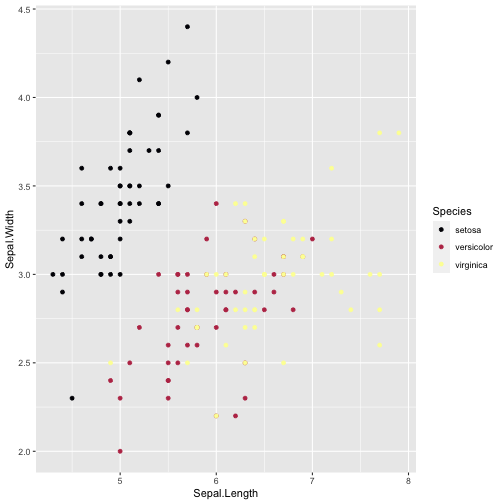<!-- --> --- ```r ggplot(iris) + geom_point(aes(x = Sepal.Length, y = Sepal.Width, color = Species, shape = Species, alpha = Species)) + scale_x_continuous( breaks = c(170,200,230)) + scale_y_log10() + scale_colour_viridis_d() + scale_shape_manual( values = c(17,18,19)) + scale_alpha_manual( values = c( "setosa" = 0.6, "versicolor" = 0.5, # "virginica" = 0.7)) ``` <!-- --> --- ## Highlight data points https://thiyanga.netlify.app/post/scatterplot/ --- 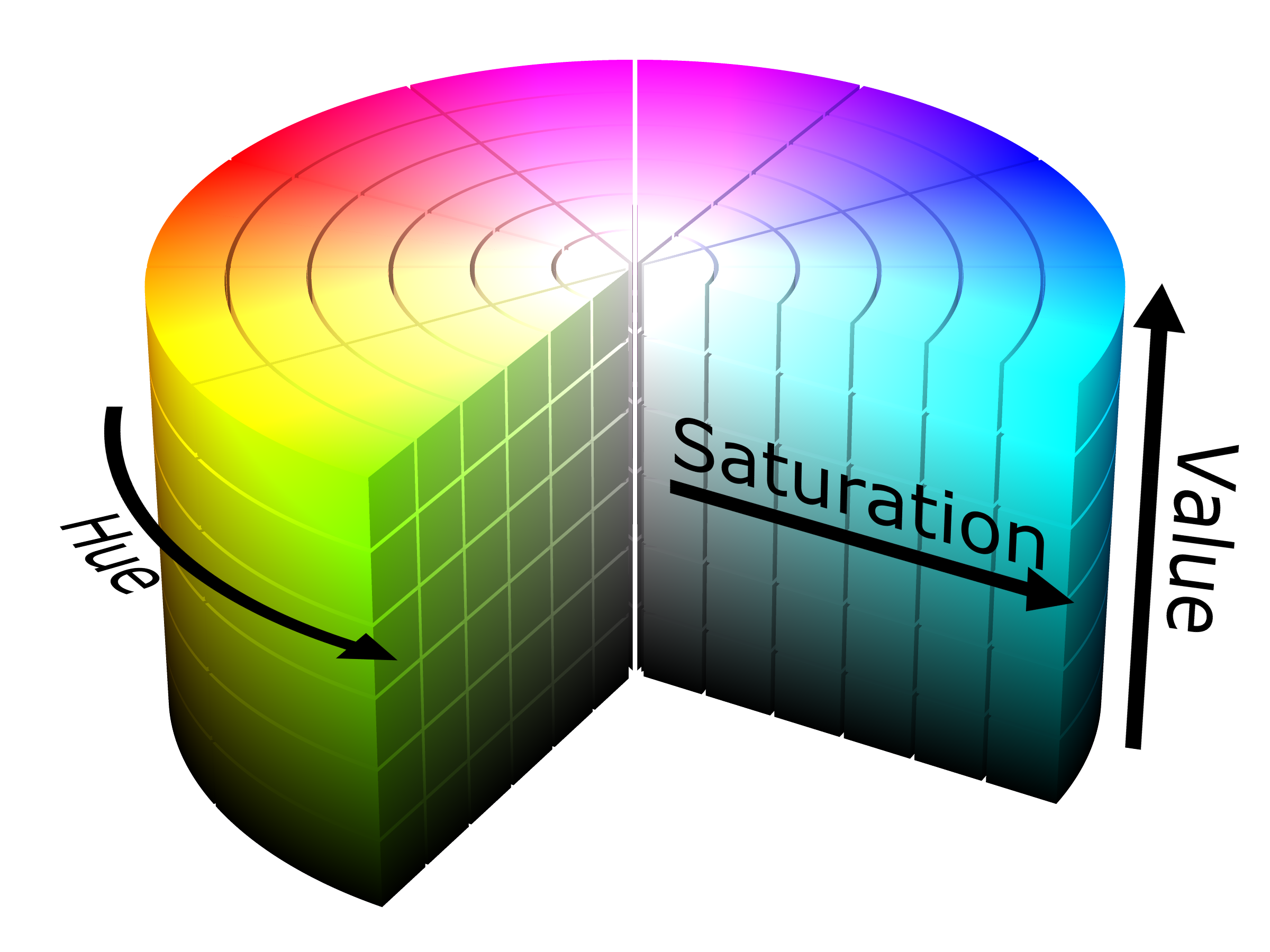 --- ## HSL colour attributes .pull-left[ 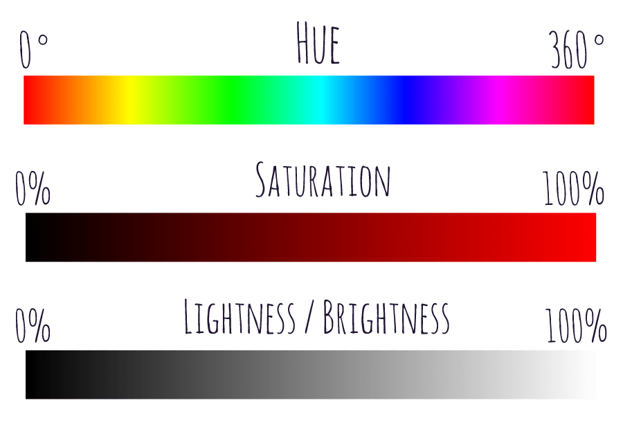 ] .pull-right[ Hue: true colours without tint or shades Saturation: light tints to dark shades Lightness (Value) ] image source: https://purple11.com/basics/hue-saturation-lightness/ --- class: inverse, middle, center # Coordinates --- ```r library(palmerpenguins) data(penguins) ggplot(penguins) + geom_bar(aes(x= species, fill = species)) ``` <!-- --> --- ```r ggplot(penguins) + geom_bar(aes(x= species, fill = species)) + coord_flip() ``` <!-- --> --- .pull-left[ ```r ggplot(penguins) + geom_bar(aes(x= year, fill = species)) ``` <!-- --> ] --- .pull-left[ ```r ## Zooming into a plot with scale ggplot(penguins) + geom_bar(aes(x= year, fill = species)) + scale_y_continuous(limits = c(0,115)) ``` ``` ## Warning: Removed 1 rows containing missing values (`geom_bar()`). ``` <!-- --> ] .pull-right[ When zooming with scale, any data outside the limits is thrown away ] --- ## Zooming into a plot with scale .pull-left[ ```r ggplot(penguins) + geom_bar(aes(x= year, fill = species)) + coord_cartesian(ylim = c(0,115)) ``` <!-- --> ] .pull-right[ Proper zoom with `coord_cartesian()` ] --- .pull-left[ ```r p <- ggplot(mtcars, aes(disp, wt)) + geom_point() + geom_smooth() p ``` ``` ## `geom_smooth()` using method = 'loess' and formula = 'y ~ x' ``` <!-- --> ] .pull-right[ ```r # Setting the limits on a scale converts all values outside the range to NA. p + scale_x_continuous(limits = c(325, 500)) ``` ``` ## `geom_smooth()` using method = 'loess' and formula = 'y ~ x' ``` ``` ## Warning: Removed 24 rows containing non-finite values (`stat_smooth()`). ``` ``` ## Warning: Removed 24 rows containing missing values (`geom_point()`). ``` 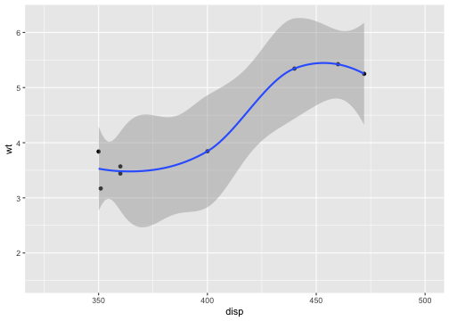<!-- --> ] --- .pull-left[ ```r p <- ggplot(mtcars, aes(disp, wt)) + geom_point() + geom_smooth() p ``` ``` ## `geom_smooth()` using method = 'loess' and formula = 'y ~ x' ``` 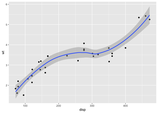<!-- --> ] .pull-right[ ```r # Setting the limits on the coordinate system performs a visual zoom. # The data is unchanged, and we just view a small portion of the original # plot. Note how smooth continues past the points visible on this plot. p + coord_cartesian(xlim = c(325, 500)) ``` ``` ## `geom_smooth()` using method = 'loess' and formula = 'y ~ x' ``` 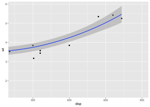<!-- --> ] --- ```r ggplot(iris, aes(y=Sepal.Length, x=Sepal.Width)) + geom_point() ``` 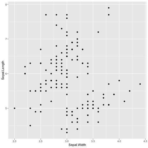<!-- --> --- ```r ggplot(iris, aes(y=Sepal.Length, x=Sepal.Width)) + geom_point() + coord_fixed(ratio = 1) ``` <!-- --> --- ```r ggplot(iris, aes(y=Sepal.Length, x=Sepal.Width)) + geom_point() + coord_fixed(ratio = 0.5) ``` <!-- --> --- ```r ggplot(iris, aes(y=Sepal.Length, x=Sepal.Width)) + geom_point() + coord_fixed(ratio = 5) ``` <!-- --> --- ```r ggplot(iris, aes(y=Sepal.Length, x=Sepal.Width)) + geom_point() + coord_fixed(ratio = 1/5) ``` <!-- --> --- ```r ggplot(iris, aes(y=Sepal.Length, x=Sepal.Width)) + geom_point() + coord_fixed(ylim = c(0, 6)) ``` <!-- -->